Project 01: GeoPINN Demo: Solving PDEs on a Sphere
Project code: projects/01-GeoPINN-Manifold__project-space
This project is best understood as a three-step story:
- Without my GeoPINN: the analytical solution of a scalar PDE on the unit sphere exists as a known closed-form mathematical expression.
- With my GeoPINN: a neural network learns the same PDE solution directly on the manifold, with no mesh and no flat grid.
- Final Taichi demo: the learned field is rendered as a rotating, gently deformed, diverging-colored sphere in Taichi GGUI.
The important point is not that the final render looks nice. The important point is that the PDE is being solved intrinsically on the manifold. The network ingests (x, y, z, t) points on the surface, and the Laplace–Beltrami operator is computed via autograd on the embedded sphere. No lat/lon grid. No pole singularities. No triangulation.
Without My GeoPINN vs With My GeoPINN
The comparison that matters is not "rough render vs polished render." It is "closed-form analytical solution vs learned PINN surrogate."
Both videos use the same camera, the same time window, and the same colormap. The scalar field on the surface is the heat equation on the unit sphere, evolving from an ℓ=2 spherical-harmonic initial condition:
- governing PDE:
∂u/∂t = Δ_S u - initial condition:
u(x, 0) = xy + 0.5 · yz - analytical solution:
u(x, t) = e^(-6t) · (xy + 0.5 · yz)
The e^(-6t) decay rate is not a hyperparameter. It is the eigenvalue of ℓ=2 spherical harmonics under the Laplace–Beltrami operator on the unit sphere. The analytical side is exact. The GeoPINN side was trained only on collocation points, a handful of initial-condition samples, and a small supervision set.
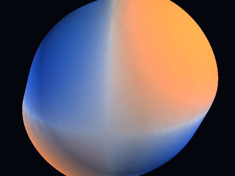
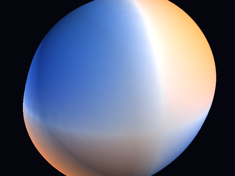
|
Without My GeoPINN Closed-form analytical solution for the heat equation on the unit sphere. |
With My GeoPINN Learned PDE solution from a 50 305-parameter MLP, same time window.
|
The left side is the target — the exact answer. The right side is a neural network that has never been told the closed form. What matters is that they look virtually identical, and the quantitative agreement below confirms that the surrogate is tracking structure rather than producing plausible-looking noise.
The side-by-side version, for a single-viewport read:
And a few matched still frames across the decay, so you can look at the field structure itself rather than only motion:
t = 0.00
|
t = 0.07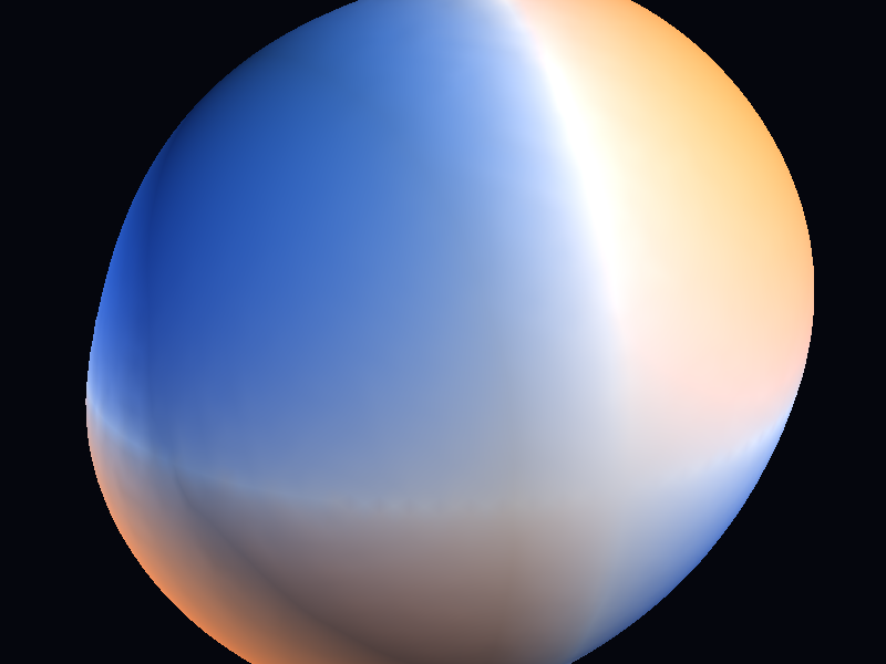
|
t = 0.15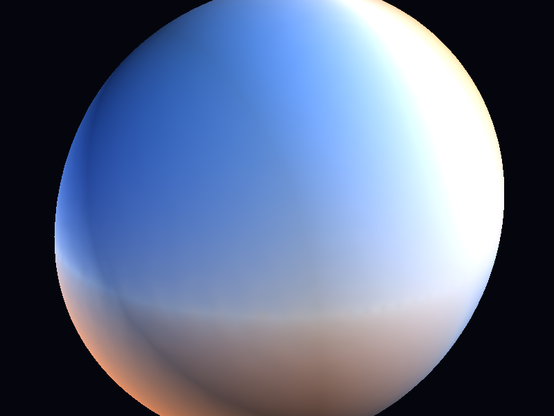

|
t = 0.20

|
Top row is analytical, bottom row is GeoPINN, at matched timesteps. By t = 0.20 the field has already decayed to about 30 % of its initial amplitude, and the two rows still agree in both structure and sign pattern.
The Manifold Angle
The manifold is the point. Everything else in this project exists to make that point visible.
Flat domains have it easy
Most introductory PINN examples solve PDEs on a flat rectangle. The Laplacian on a flat domain is the familiar Δu = ∂²u/∂x² + ∂²u/∂y² + ∂²u/∂z², and you can just autograd your way to it.
On a curved surface, that is not the operator you want. A sphere is not flat, and the relevant differential operator has to respect the intrinsic geometry.
The Laplace–Beltrami operator, plainly
The Laplace–Beltrami operator Δ_S is the sphere-native replacement for the flat Laplacian. Informally:
Δ_S umeasures how much the value ofuat a point differs from the average ofuin a small geodesic neighborhood on the surface, using the surface's own notion of distance rather than the ambient 3D notion.
For a smooth function u defined on a surface embedded in 3D, there is a concrete formula that makes this computable without ever leaving the embedding:
Δ_S u = Δu − n · ∇(n · ∇u) − (n · ∇u) · (∇ · n)
where n is the unit normal to the surface and Δ is the ordinary 3D Laplacian. The key property is that Δ_S u only depends on how u varies along the surface — motion off the surface is projected away.
That is exactly what autograd gives you. The network eats (x, y, z, t), and the loss computes Δ_S u_θ by taking 3D derivatives and removing the normal component. No mesh. No stencil. No pole patch.
Why this matters beyond the sphere
The sphere is the demo, not the point.
Everything in this pipeline generalizes to any smooth Riemannian manifold where you can compute a surface normal or have an atlas. That includes:
- tori (coolant loops, topological shells)
- ellipsoids (planetary climate, non-spherical bodies)
- arbitrary triangulated surfaces (CAD geometry, brain cortex, fabric)
- implicit surfaces (signed distance fields, level sets)
Solving PDEs on those geometries with classical methods is where things get painful. Lat/lon grids break at the poles. Cubed-sphere grids introduce artificial seams. Unstructured meshes force you to rewrite operators. The GeoPINN formulation sidesteps all of that by staying intrinsic.
That is the structural claim of the project:
Replace "discretize the domain, then solve the PDE" with "query the manifold pointwise, then ask the network to satisfy the PDE there."
Visual Design Choices
A static plot of a scalar field on a sphere, unrolled to a 2D rectangle, throws away the thing that makes the problem interesting: the field lives on a curved surface.
The Taichi viewer is structured so the geometry reads immediately.
Diverging colormap, tanh transfer
The field u(x, t) is signed — it has roughly equal positive and negative lobes from the ℓ=2 harmonic. A single-hue colormap would waste half the dynamic range.
- positive values map to a warm orange
- negative values map to a cool blue
- the midpoint is a neutral background tone rather than pure white, so the sphere keeps depth
Before colormapping, each frame is normalized against the 99th percentile of absolute amplitude, then pushed through tanh(normalized · gain) with gain = 2.4. The tanh transfer does two useful things at once:
- compresses outliers so a single hot point cannot dominate the hue scale
- amplifies mid-range structure so the
ℓ=2lobes stay crisp even as the amplitude decays
Without the tanh compression, the late timesteps would read almost entirely neutral because the global amplitude has already decayed to about 30 %. The transfer function keeps the shape of the field legible while honestly signaling the scale of it through deformation.
Radial deformation, on purpose
The sphere in the viewer is not perfectly round. Each vertex is pushed outward along its normal by an amount proportional to the local field value.
- amplitude
0.06at thepitchpreset - amplitude
0.09at thedramaticpreset - amplitude
0.05at theresearchpreset (wireframe visible, so less deformation is needed)
This matters because color alone tells you the sign of the field. Radial deformation gives you a second channel for magnitude. Two peaks the same color can still be visually separated by how much they push the surface outward. At a glance, you see where the field is strong and which way it is pointing without reading a legend.
It also does one rhetorical job: the sphere visibly breathes as the field decays, which makes the physics of the heat equation readable as motion rather than as a fading color.
Why sphere over flat plot
A heatmap on a flat plane would show the same numbers, but it would hide the structural claim of the work. The point of a Geo-PINN is that the network learned the field on a curved domain. Showing the field on its actual domain is not presentation fluff — it is a direct statement about what was solved.
Metrics
Honest numbers first.
- mean L2 error (vs analytical):
4.92e-3 - mean PSNR:
47.16 dB - final PDE residual:
4.58e-4 - final IC loss:
4.45e-5 - relative L2 error, averaged across the time window:
3.3 % - relative L2 error, worst single timestep (t=0.20):
5.1 % - training time: about
38 son an RTX 3090 Ti - model size:
50 305parameters, 4-layer MLP, hidden128, tanh activations - evaluation set:
15 000dense points ×12timesteps, sampled uniformly on the sphere
The error rises slightly with t. That is partly because the absolute amplitude decays, so the same absolute error becomes a larger relative percentage, and partly because the supervision signal thins out as the field flattens. A 5.1 % relative L2 at the latest timestep is the honest ceiling on fidelity for this configuration — not the average.
The PDE residual at the end of training is about 4.58e-4. That is the thing the network was actually being asked to minimize pointwise. It is small enough to mean the trained field is close to satisfying the heat equation on the manifold, not just close to the training samples in value.
Preset Showcase
Three deliberate presets rather than one accidental look.
|
Research Wireframe on, equatorial camera, restrained deformation. The "proof that the field is really on a sphere" view. 
|
Pitch Oblique camera, warm key light, smooth diverging colormap. The default hero-shot preset. 
|
Dramatic Close camera, strong contrast, more deformation, faster rotation. The cinematic sell. 
|
The default preset is Pitch because it keeps the comparison legible without drifting into the busier look of research or the tighter, higher-deformation framing of dramatic. In the interactive viewer, [ and ] cycle between them.
Why It Matters
Here is the strongest way to frame the project:
This work solves a PDE on a curved manifold using a neural network that has no notion of a mesh, no pole singularities to patch, and no per-geometry stencil rewrite.
That matters for a few reasons.
1. PDE solving becomes geometry-agnostic
Classical PDE solvers on curved surfaces need surface-specific machinery. Spectral methods need a basis suited to the geometry. Finite differences need a structured grid that the sphere does not admit without artifacts. Finite elements need a mesh, and a good mesh on a complex surface is its own research project.
GeoPINN needs none of that. The network queries the surface pointwise. The PDE residual is computed via autograd. The only thing that changes between a sphere and a torus is the normal vector field. That is the representation shift.
2. The solution is a continuous field on the manifold
The analytical side gives you a formula. A classical numerical solver gives you a mesh of samples. GeoPINN gives you a callable function u_θ: (x, y, z, t) → u, evaluable at any point on the surface and any time in the training window.
That means the Taichi viewer can query the trained checkpoint at 10 242 vertices of an icosphere, or at a completely different resolution, without rerunning anything. Rendering decouples from solving.
3. One checkpoint drives the whole pipeline
One 50 305-parameter .pt file now drives:
- side-by-side comparison clips against the analytical solution
- per-timestep snapshot exports
- three Taichi presets at arbitrary camera angles
- the interactive viewer with preset cycling
That is the workflow win. Solving the PDE once produced a compact reusable object that feeds validation and presentation without re-invoking the physics pipeline.
4. The Taichi viewer is a stress test, not just polish
Rendering the field on its actual curved domain is useful because a sphere exposes problems. If the learned field were incoherent across hemispheres, the rotation would make that visible immediately. If there were seam artifacts from a sloppy parameterization, the viewer would show them. If the residual had pole bias, the poles would flicker.
The fact that the sphere rotates cleanly, the decay reads continuously, and the sign pattern stays stable across the full time window is evidence that the learned representation is intrinsically coherent on the manifold — not just coherent on a specific evaluation grid.
What Would Make This More Realistic
The current result is strong enough as a geometry-aware PDE demo, but it is still not the strongest possible version of a learned manifold PDE system.
The main realism limit is that the target PDE is a relatively clean linear problem on the cleanest possible closed manifold. The demo is correct about what it shows — it does not yet show what happens when the geometry, the PDE, or the initial conditions get genuinely hostile.
Realism has to improve across the whole stack
For this project, realism is a layered problem:
- Target PDE richness: the heat equation is linear and globally decaying. Real geophysical problems include advection, coupling, and nonlinear coupling terms.
- Geometry: the unit sphere has a closed-form normal field everywhere. Arbitrary triangulated surfaces or SDF-defined geometries are much less forgiving.
- Operator discretization: the intrinsic Laplace–Beltrami via autograd is elegant, but more complex operators (covariant derivatives of vector fields, Hodge Laplacians) need more care.
- Temporal horizon: the demo runs on a short window
t ∈ [0, 0.2]. Longer horizons test whether the learned dynamics stay coherent far from the IC. - Evaluation: agreement with the analytical solution is the strongest possible evaluation, but it only exists because the PDE was chosen to admit one.
If any of those layers stays simple, the project reads as a demonstration rather than as a general-purpose method.
1. Move to a PDE with no closed-form solution
The honest next step is a PDE where an analytical baseline does not exist. Shallow-water equations on the sphere are the obvious choice — they are nonlinear, they couple height and velocity fields, and they are the standard atmospheric-dynamics benchmark. Evaluating GeoPINN against a high-order classical solver rather than against a closed form is a more realistic test of the method.
2. Move off the sphere
The whole structural claim is that the method generalizes to arbitrary smooth manifolds. Proving that claim means actually running it on:
- a torus (genus-1 test)
- an ellipsoid (broken symmetry, locally varying curvature)
- a triangulated mesh (surface normals from vertex normals, not from a formula)
- an implicit surface (normals from the SDF gradient)
Each of those introduces a different realism test. The torus exposes topology. The ellipsoid exposes anisotropy. The mesh exposes discretization of the normal field. The implicit surface exposes differentiation across the zero level set.
3. Harder initial conditions
The current IC is a single ℓ=2 spherical harmonic, which has a known eigenvalue under the Laplace–Beltrami operator and therefore admits an exact solution. Richer realism comes from:
- superpositions of multiple harmonics at different scales
- localized sources (Gaussian bumps, delta-like spikes)
- discontinuous ICs that test whether the learned field smears or stays sharp
- random ICs drawn from a Gaussian random field on the sphere
4. Longer horizons
The demo runs t ∈ [0, 0.2] because that is where the ℓ=2 harmonic still has readable amplitude. For the heat equation that is fine, but longer horizons would test whether the model preserves structure near equilibrium, where gradients become small and supervision signal vanishes.
5. Nonlinear PDEs
The heat equation is linear. The real argument for neural PDE solvers is strongest on nonlinear PDEs where classical methods struggle. Extending the GeoPINN formulation to:
- reaction-diffusion (Fisher-KPP, Allen–Cahn on the sphere)
- viscous Burgers on the sphere
- shallow-water or geostrophic turbulence
- Navier–Stokes on a curved domain
would turn the demo from a proof of concept into a method with teeth.
If I compress the realism roadmap to one line, it is this:
The path to a more realistic GeoPINN is harder PDEs on less forgiving manifolds with less supervision, validated against actual numerical baselines rather than closed-form solutions.
If I Were Continuing This Project
If I had another serious pass on GeoPINN rather than just polishing the current milestone, I would prioritize the work in this order.
Priority 1: non-spherical geometry
The single highest-leverage next step is running the same training and rendering pipeline on a non-spherical surface. That is what cashes in the "works on any smooth manifold" claim. A torus or an ellipsoid would be the right first target.
Priority 2: a PDE with no closed-form baseline
After that, I would move to shallow-water or reaction-diffusion on the sphere, evaluated against a high-order classical solver. This is the move from "correctness on a toy problem" to "competitive against real baselines."
Priority 3: longer time horizons and richer ICs
Once the method is producing credible solutions on harder PDEs, the next move is stress-testing temporal coherence and IC diversity.
Priority 4: presentation refinements
Only after the above would I spend more time on:
- multi-field visualization (height + velocity for SWE)
- better normal-aware shading on non-spherical surfaces
- time-scrubbable interactive viewers
- clearer labeling and legend overlays
Those matter, but they are downstream of the physics.
Honest Current Limitations
The main current limitations are:
- only one PDE (heat equation on the unit sphere) is demonstrated
- the initial condition is a single spherical harmonic, chosen because it admits an exact solution
- the time horizon is short (
t ∈ [0, 0.2]) and the relative error grows witht - evaluation is against the closed form, not against another numerical solver
- the manifold is the cleanest possible closed manifold
None of those invalidate the project. They define its current scope.
If I reduce the whole post to one sentence, it is this:
The value is not that the sphere looks nice in Taichi. The value is that the PDE was solved on the manifold, pointwise, with no mesh — and the final render is evidence that the learned field is intrinsically coherent enough to rotate cleanly.