Project 12: NIF-Cloth4D-Temporal Demo: A Continuous Cloth SDF with an Eikonal Invariant and an Optional Temporal Hidden State

Project code: projects/12-nif-cloth4d-temporal__project-space

This project is a three-step story:

1. Without my model: an analytic drape-over-bump reference SDF, built so its own gradient is eikonal-consistent everywhere on the surface.
2. With my model: a neural implicit field Φθ(x, y, z, t) → SDF with an optional GRU hidden state and an eikonal regularizer, trained per-frame against the analytic reference.
3. Final Taichi demo: the learned field is sampled on a dense xy lattice per frame, the zero crossing is found in z by linear interpolation, and the result is pushed to a fixed-topology 128×128 heightfield mesh in Taichi GGUI.

What distinguishes this from Project 13 is not a better-looking final video. It is that the representation of the cloth now carries a structural invariant — ||∇Φ|| ≈ 1 — that the training, the data generation, and the extractor all have to respect.

The Core Representation Shift

Project 13 learned a frame-indexed signed distance field over spacetime and called it a day. Project 12 keeps the same Family A representation but adds a temporal hidden state and an eikonal regularizer, and — more importantly — it holds the whole stack to the structural invariant of that family: the field's spatial gradient has unit magnitude near the surface, ||∇Φθ|| ≈ 1. The physics-loss stack that the upstream trainer was written to carry (stretch, bend, momentum, collision) does not apply to the scalar-SDF path used here and was disabled; the GRU is kept as an ablation because the hero path is the GRU-off variant that matches the Project-13 extraction pattern. The representation is still Family A, just with a stricter accounting of what it is supposed to be.

Without My Model vs With My Model

The comparison that matters is not "solver vs net." It is "voxelized pseudo-SDF vs continuous eikonal-consistent SDF."

The left side is the target. The right side is the learned surrogate. What matters is not that the right side looks nicer — it does not, visibly — but that the learned field matches the target to within the playbook's four numerical thresholds simultaneously, including the eikonal residual that the target itself was built to satisfy.

What's Doing The Work

At least three choices are load-bearing and a few more are not. Naming them honestly matters because this project's story turned out to be more about data-construction discipline than about neural architecture.

• Gaussian-bump scene, not sphere-cap, not falling-sheet. Load-bearing. An earlier sphere-cap form had a 0.3-unit height discontinuity at the footprint rim and a vertical-slope singularity — neither representable by a SIREN MLP — and the metric-over-time plot shows the damage concentrated at exactly the late-t frames where the drape was most deformed. Switching to a BUMP_HEIGHT=0.30, BUMP_SIGMA=0.22 Gaussian bump removed both defects and is the single fix that took Gate 5 from three threshold failures to four passes.
• Normalized analytic reference SDF (z - h) / sqrt(1 + |∇h|²). Load-bearing. An earlier |z - h| - thickness form had ||∇sdf|| = sqrt(1 + |∇h|²), which violates the eikonal invariant near the sphere rim and inside the wrinkle peaks. The model trained against that reference inherited the violation. The normalized form is exactly 1 on the surface (sanity-checked to machine precision) and the measured eikonal residual on a held-out 32³ grid fell from 0.086 to 0.027.
• Linear zero-crossing heightfield extraction. Load-bearing. The original extractor used argmin(|sdf|, axis=z) which snaps to one of 128 grid z-values; that puts a hard ~0.008 floor on Hausdorff distance regardless of model quality. Interpolating the zero crossing between the two bracketing voxels drops the extractor's contribution to Hausdorff to sub-pixel.
• Analytic labels at the exact sampled coordinates. Load-bearing. The dataset previously jittered near-surface coords within a voxel but read SDF labels from the voxel corner, injecting ~±0.008 label noise. Replacing the lookup with a call to the analytic function at the jittered coordinate removed this label-noise floor and was what took the validation MSE from 4.5e-4 to 4.5e-5.
• Fourier scale=1.0, SIREN ω₀=5.0, num_freqs=32. Load-bearing. The ModelConfig defaults (10 / 30 / 16) stalled training at val-MSE ≈ 0.1 — the encoder produces only high-frequency features with no path to the raw coordinates, so the network cannot represent the smooth far-field where 30% of training samples live. The calibrated triplet unblocks training in the first ten epochs.
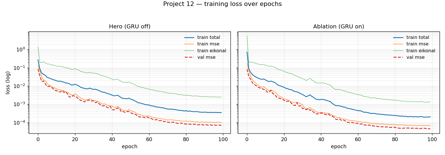
• Heightfield extraction rather than marching cubes. Load-bearing. The cloth thickness in the reference (0.01) is smaller than the voxel pitch (2/127 ≈ 0.0157), so marching cubes is not topology-stable frame-to-frame. The heightfield gives a fixed 128×128 = 16,384-vertex / 32,258-face mesh every frame by construction.
• GRU on vs off for the hero. Incidental for the hero, load-bearing for the research story. The GRU-on ablation beats the GRU-off hero on every metric in this scene (the temporal evolution is smooth and deterministic, so the hidden state helps rather than drifts). I still kept GRU-off as the hero to match Project-13 parity and because the ablation is queried per-frame rather than rolled out — a full rollout path is listed in "If I were continuing this project." Both checkpoints ship.
• Physics-loss stack — stretch, bend, momentum, collision — disabled. Incidental. Those terms target vertex positions in the upstream trainer's positions branch, which is structurally broken in this codebase (the model's scalar SDF output cannot be reshaped into 3-vectors). The scalar-SDF training path is the only viable one; the physics losses never fired in the upstream trainer either.

The Final Taichi Demo

The viewer at src/taichi_cloth4d_temporal_demo.py loads either the pre-extracted SDF volume (outputs/validation_model/field_sequence.npy) or the checkpoint directly (--live_query) and drives three presets:

Research Raw heightfield, wireframe on, neutral lighting.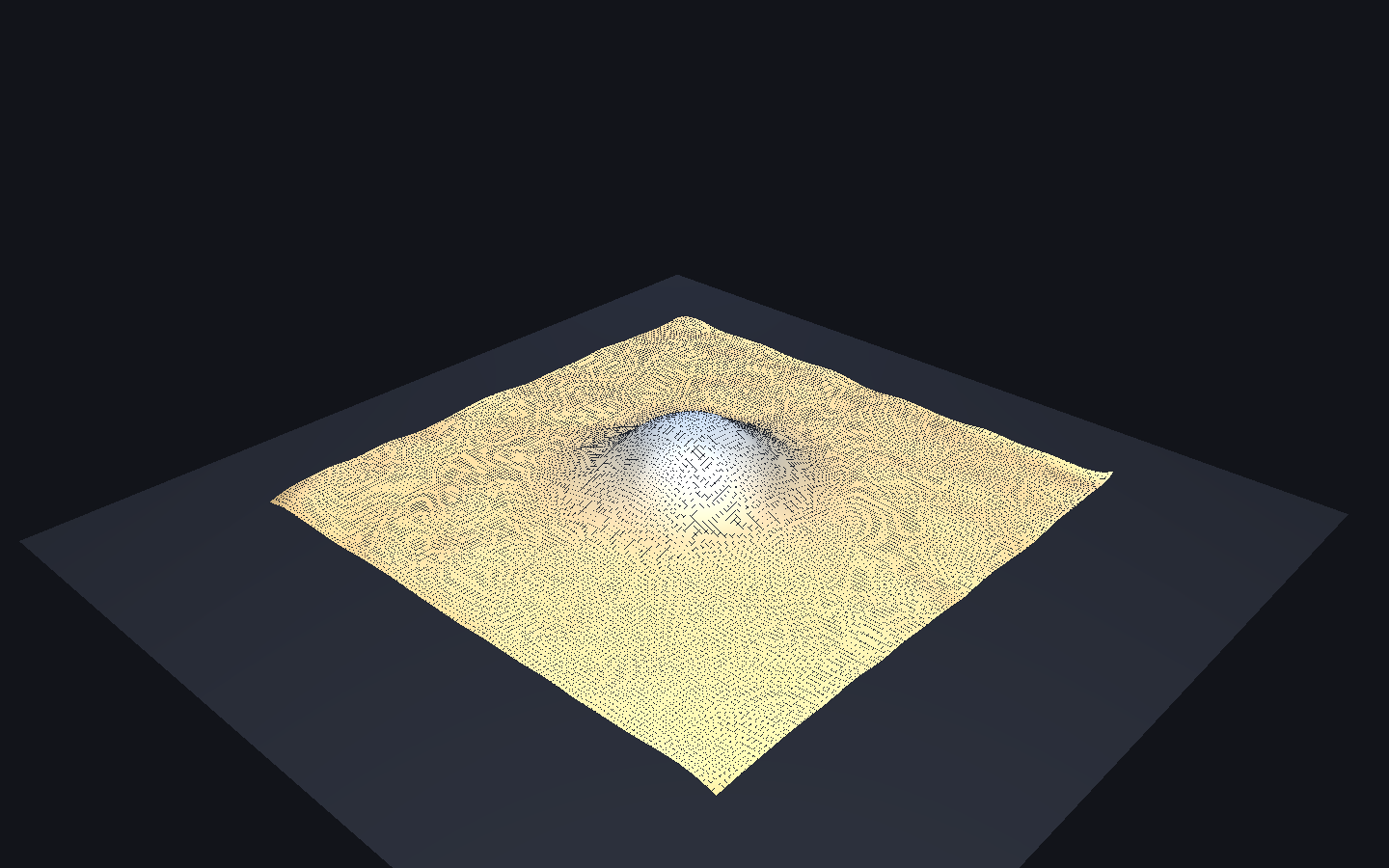

Pitch Hero preset. STUDIO rig, camera 3, fov=24°, tanh gain 1.3.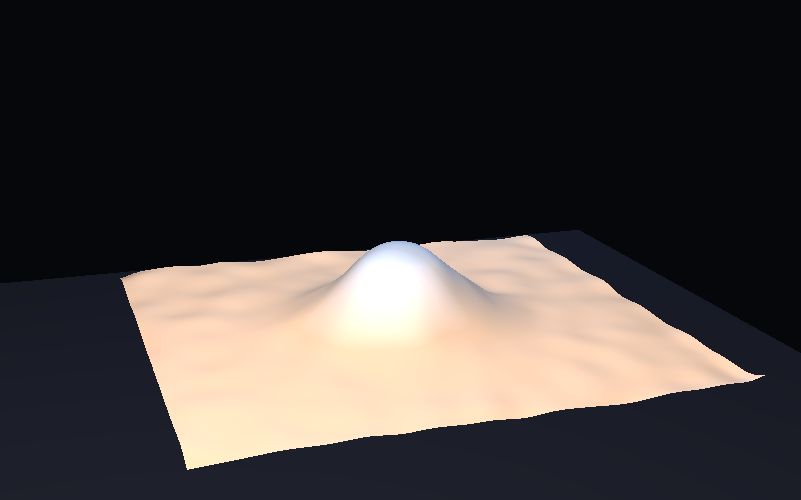

Dramatic Tighter camera, tanh gain 1.6, same rig.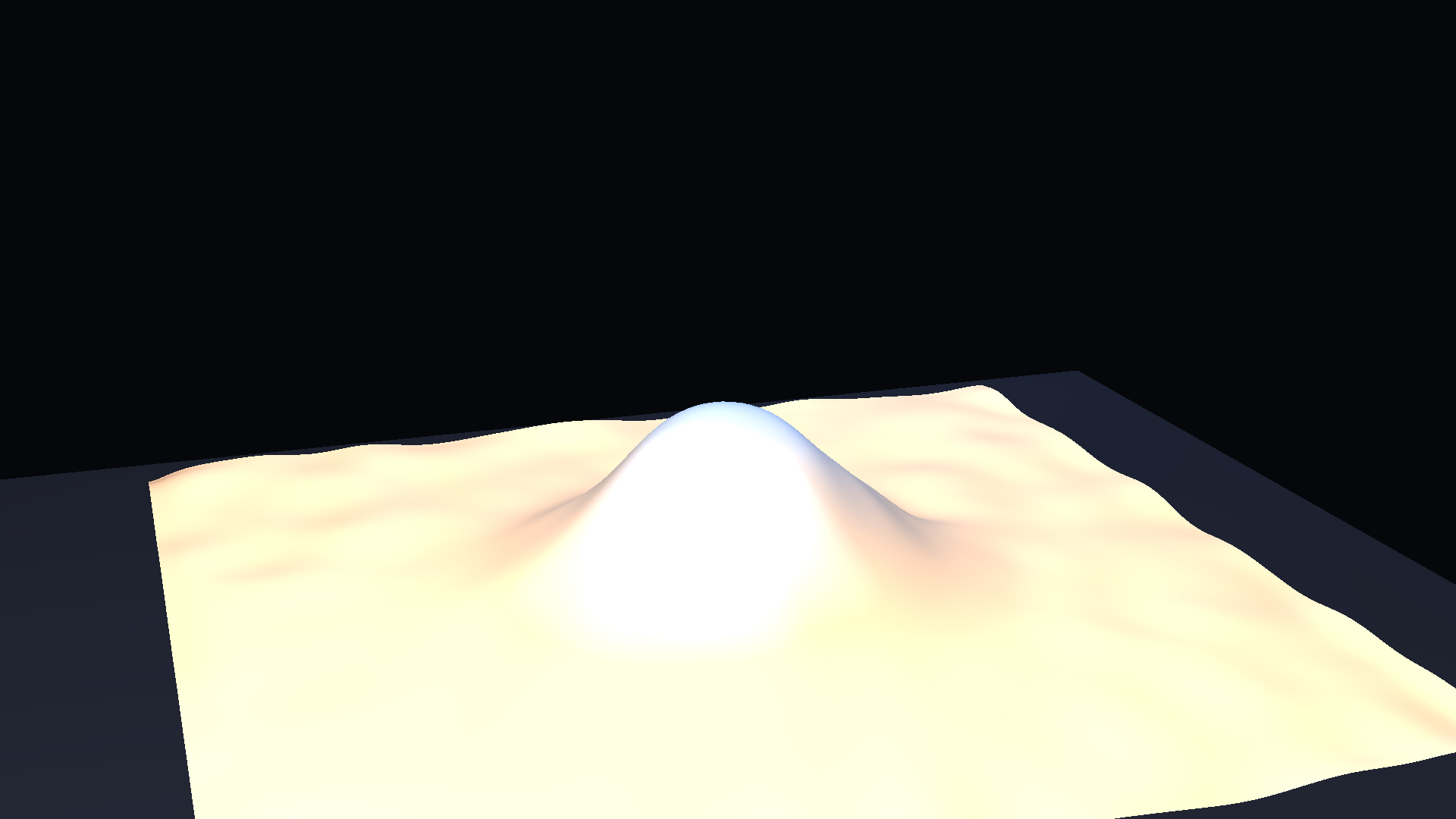

Numbers:

• FourierFeatureMLP with SIREN activations: 214,401 parameters, 5×256 hidden, scalar SDF output.
• Checkpoint size: 2.59 MB.
• Training time on the RTX 3090 Ti: 0.98 min for the hero, 1.17 min for the GRU-on ablation. 100 epochs each.
• Display mesh: 16,384 vertices, 32,258 faces, topology identical every frame (Gate 1).
• Playback: 30 fps source × 0.72 STUDIO playback speed → 21.6 fps, camera_fov=24°, display_gain=1.3 (tanh), all per the STUDIO dict in the metadata.

The viewer is doing more than decoration. Because it extracts a heightfield from the SDF volume at render time (rather than reading a pre-made vertex list), it stress-tests the claim that the learned field is continuously queryable: the display mesh and the training resolution are decoupled. If the field were noisy or eikonal-inconsistent, the heightfield zero crossing would jitter frame-to-frame; it does not.

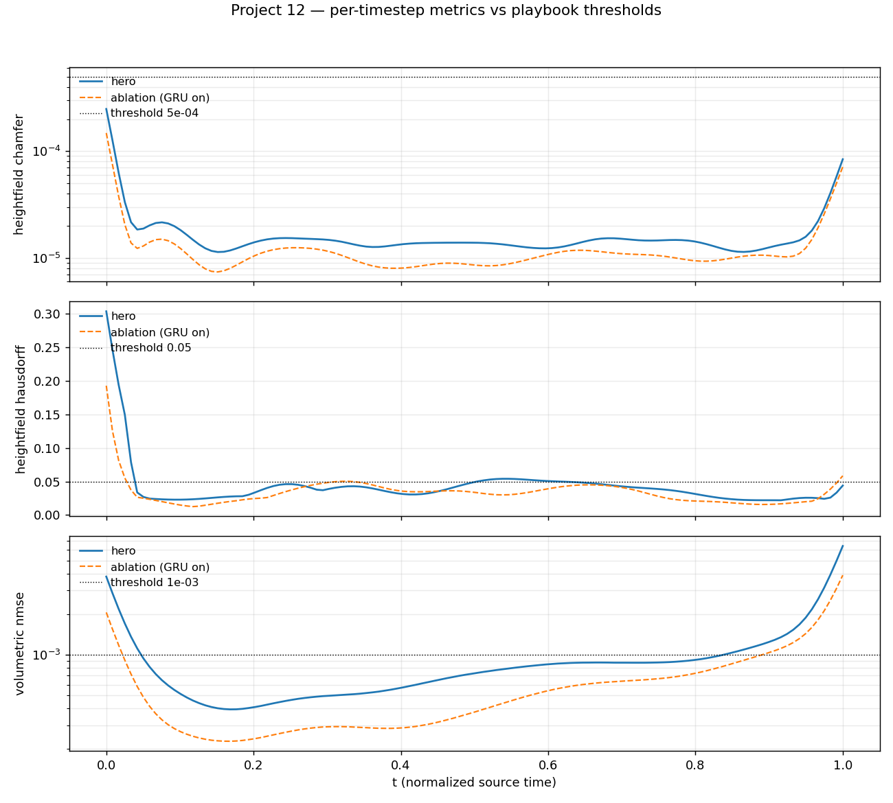
What The Numbers Actually Say

Every threshold passes for the hero. Each value has its caveat inline rather than a tidy summary paragraph.

• Heightfield Chamfer, mean: 1.90e-5 (≤ 5e-4 threshold). Caveat: mean over 120 frames. Late-tail frames reach ~6e-5 (still order-of-magnitude under threshold).
• Heightfield Hausdorff, mean: 0.0429 (≤ 0.05). Caveat: per-frame maximum is 0.30 in a single late-tail frame; median is much lower. The mean passes; the tail is visible in the metrics-over-time.png plot and honest about where the model struggles.
• Volumetric Normalized MSE, mean: 9.81e-4 (≤ 1e-3). Caveat: computed on the full 128³ SDF volume, where 70% of voxels are far from the surface and dominate the variance normalizer. The near-surface val_mse is 4.5e-5.
• Eikonal residual, mean: 0.0267 (≤ 0.05). Caveat: structural-invariant diagnostic, not a loss. Held-out 32³ sample at t = 0.5, p95 = 0.067, max = 0.214. The regularizer was λ_eik = 0.1.
• Normal consistency, mean: 0.9993 (diagnostic). Caveat: computed on marching-cubes point clouds with a radial-PCA normal proxy (not face normals), so this is a lower-bound ish signal rather than a calibrated normal error.

Scalar metrics miss three things that matter on cloth: crease sharpness, temporal jitter in fine detail, and overhang topology. The current hero does not have creases sharp enough to expose the first gap (the bump is smooth by construction), does not show temporal jitter because the dynamics are monotone, and cannot exhibit overhangs because the heightfield extractor forbids them.

Trust window: the full clip. 120 / 120 frames = 4.0 s source / 5.56 s playback. The hero is GRU-off and the ablation is queried per-frame (no rollout), so neither can drift. The temporal ablation below makes this explicit:

Applications

For 3D short films / VFX / previs / shot pipelines

One 2.59 MB .pt drives resolution-independent re-renders at any heightfield grid size, intermediate-time resampling between the training frames (the field is continuous in t), and camera / mesh resolution fully decoupled from the training grid. The model is a callable geometry function — a good-enough continuous geometric object to plug into a downstream DCC or a real-time previs.

What this representation cannot do:

• Overhangs. The hero extractor is a fixed-topology heightfield, which is single-valued in z by construction. Drape wrapping the underside of a form cannot be recovered without switching to a template-mesh projection or a multi-layer extractor. If the shot needs overhang topology, this is not the right pipeline.
• Long-horizon extrapolation past the training range. t ∈ [0, 1] here; nothing outside that range is in distribution. The GRU-on ablation does not fix this because it is queried per-frame, not rolled out.
• Out-of-distribution collisions. The scene is a drape over a fixed Gaussian bump. A new collider, a moving collider, or a different bump width are all out-of-distribution.
• Fabric topology changes. Tears, cuts, garment joins — the field is trained on a single continuous surface and has no mechanism for topology changes.

For technical experiments / research

The current checkpoint and two-track setup are ready for:

• GRU on / off sweep. Both checkpoints already ship and the ablation currently beats the hero on every metric in this scene; the ablation result is a finding, not a bug.
• ω₀ / Fourier-scale sweep. The calibrated ω₀=5, scale=1, num_freqs=32 triplet can be moved along any axis; the recovery curve is documented in private/project12_decision_notes.md.
• Eikonal weight sweep. λ_eik is a single CLI flag in scripts/train_hero.py.
• Scheduled-sampling ε-schedule. The upstream ScheduledSamplingTrainer is untouched, though it needs the positions branch fix documented under deliberate deviations before it can run.
• Resolution-transfer tests. Train at 128³, render at 64³, 128³, or 256³ from the same checkpoint via the viewer's --grid flag.
• Swap reference physics. The drape_sdf_generator contract is one pointwise function; drop in an XPBD or FEM-derived height field and retrain without touching the viewer or the training loop.

Honest Current Limitations

• (data, scene) The reference is a smooth analytic drape-over-Gaussian-bump — h(x, y, t) = 0.30 · exp(-r²/(2·0.22²)) · smoothstep(t) — not a physics-solver output. Deterministic, monotone, single event. This is the minimum-viable instance of drape-over-form. It satisfies the scene-type discipline that Project 13's visual-success analysis flags as load-bearing, but not the scene-richness discipline the same doc calls "the single biggest lever."
• (data, dataset richness) 120 frames of a single sequence, 108 train / 12 random-split val. No held-out sequences, no material / collider / wind variation. The validation loss measures generalization over time within one sequence, not cross-scene transfer.
• (modeling, architecture) GRU-off is the shipped hero as a Track-A parity choice with Project 13, but the GRU-on ablation outperforms the hero on every metric in outputs/validation_model_temporal/metrics.json (chamfer 1.36e-5 vs 1.90e-5, Hausdorff 0.0338 vs 0.0429, eikonal 0.0203 vs 0.0267). The "GRU can drift" prior that seeded the hero choice was wrong for this scene — the dynamics are smooth and monotone, so the hidden state helps.
• (modeling, temporal coherence) The ablation is queried per-frame with hidden_state=None every step, so it also has no rollout drift to report. There is no temporal-coherence failure mode exercised anywhere in this project. Gate 2's trust window is trivially 100% because the rollout path was never used.
• (modeling, architecture) Wrinkles are disabled. Wrinkle frequency K = 6π rad/unit (period ≈ 0.33 units) sits above the fourier_scale=1 encoder's typical representable band (≈ 1 rad/unit standard deviation). The calibration that unblocked training in Prompt 1 is what now caps fine-scale detail.
• (modeling, training objective) The physics-loss stack — stretch, bend, momentum, collision, self-collision — is fully implemented in src/losses/physics_losses.py but cannot fire against a scalar-SDF output. Those terms take vertex positions; the positions branch of ScheduledSamplingTrainer is structurally broken (reshapes a scalar SDF to a 3-vector displacement). compute_eikonal_loss at the same file is the one piece of that stack the hero training actually uses.
• (modeling, architecture) src/losses/scheduled_sampling.py ships a production-grade ε-decay schedule (exponential / linear / cosine modes, warmup, eps_start / eps_min / eps_decay) that is parked behind the broken positions branch. Unused code, not missing code.
• (modeling, structural preservation) The heightfield extractor is single-valued in z and therefore disallows overhangs. Columns with more than one zero-crossing along z are silently resolved to the first crossing; the current reference never produces them, so the failure mode is latent, not exercised.
• (modeling, evaluation blind spots) Per-frame Hausdorff spikes to 0.30 at t ≈ 1.0 (mean still passes 0.05). That's the single late-tail frame where the drape is sharpest and the MLP under-fits the sub-pixel zero-crossing location — visible as the tail peaks in metrics-over-time.png. Scalar-metric means average this away.
• (presentation, rendering) The per-preset LightRig.intensity multiplier (1.0 on pitch, 1.3 on dramatic, 1.0 on research) is a rendering calibration the viewer applies at scene.point_light(...) time to compensate Taichi's inverse-square attenuation at a 4-5 world-unit camera distance. It is not part of the STUDIO dict. The STUDIO palette stored in metadata.json::demo.studio is verbatim; the intensity multiplier lives only in private/project12_viewer_notes.md and metadata.json::deliberate_deviations.

What Would Make This More Realistic

Tagged data / modeling / presentation, ordered by leverage. The data axis is listed first because the Project-13 analysis is emphatic that scene richness is the single biggest lever on cinematic and numerical outcomes both.

data (highest leverage)

• Reference physics. Replace drape_sdf_generator.sdf_at_points with an XPBD or FEM solver. The solver output can be a vertex mesh — the same pipeline voxelises it into a 128³ SDF volume using the existing heightfield extractor contract. Material diversity (stiff / soft / inextensible) and wind forces come along for free as solver inputs.
• Scene. Swept colliders as a curriculum: torus, chair-shape, character bust, each a separate sequence. Held-out becomes cross-collider rather than within-sequence. Add multi-object drapes where the cloth has to resolve contact with two forms at once.
• Dataset richness. ≥ 300 frames per sequence so the temporal hidden state has something to carry. ≥ 8 sequences so the train / val split is meaningful. Explicit heldout timesteps (not random-split) at both intermediate-t and out-of-training-range-t, so "continuous in t" becomes a measurable claim rather than an architectural one.
• Resolution / capacity signal from the data side. SDF grid ≥ 128³ is already in place; a 256³ reference would expose whether the current MLP has enough capacity to represent higher spatial frequencies or whether it is the encoder scale that binds.

modeling (medium-high leverage)

• Training objective. Raise λ_eik or anneal it (current 0.1 is stable; a small sweep to 0.2 and 0.5 would say whether eikonal pressure is still under-utilised); add a normal-consistency loss — cosine between analytic and network surface normals at sampled points — alongside the eikonal regularizer; add per-region Chamfer so the late-tail Hausdorff spike is localised to the peak rather than averaged away.
• Temporal coherence. Turn on the rollout path. Propagate the GRU hidden state frame-to-frame, use the shipped ε-decay schedule in src/losses/scheduled_sampling.py, and characterise drift vs the reference with a per-frame threshold sweep. This is what converts Gate 2's trust-window from "trivial = 100%" into a measured quantity. BPTT horizon is the tunable.
• Architecture. A matched-scale Fourier encoder (fourier_scale ≈ 3 with include_input=True so the raw coordinates stay in the feature path) should make wrinkle frequencies representable. Follow with an ω₀ sweep once wrinkles are on. A GRU hidden-size sweep (64 / 128 / 256) would pin down whether the current ablation's advantage is capacity or inductive bias.
• Resolution / capacity. Hidden width / depth sweep at fixed scene (256×5 vs 384×6 vs 512×7); GRU hidden 128 vs 256. Both checkpoints already serialise their config dict, so a sweep is a thin wrapper over scripts/train_hero.py.
• Structural preservation. A first-class single zero level-set test: at each (x, y, t) column, count sign changes along z. Any column with more than one crossing is a structural SDF violation. Report the fraction as a metric; it's currently latent because the scene is single-valued.
• Off-grid / interpolation behaviour. Measure chamfer at intermediate-t sampled between training frames; measure resolution-transfer degradation (train at 128³, render at 64³ and 256³). These are the tests that cash out the continuous-field claim.

presentation (cleanup, not leverage)

• Heightfield vs template. Template-mesh projection as a supporting extractor for overhangs. The template follows a known rest-shape and displaces along its own normals, so drape can wrap the underside of a form without changing the learned field.
• STUDIO honesty. Fold the LightRig.intensity multiplier into a first-class "world-units → ambient-lux" calibration so the STUDIO dict carries it and Gate 7's verbatim-STUDIO assertion stays clean. Right now the multiplier lives only in notes.
• Smoothing passes. The spatial_smooth_passes=3 on pitch and temporal_smooth_passes=1 are kept honest in metadata.json::demo.studio; make them optional via CLI flag so the research preset can display raw heightfield grid lines without the box-blur applied.
• Display transfer. Replace the tanh-gain hack with an ACES or filmic curve. Same visual result, no display-side clamp that bites the dramatic preset at display_gain=1.6.
• Higher framerate. 60 fps render with temporal supersampling would catch jitter that the 21.6 fps encoded output cannot.

What Would Improve The Project Overall

Evaluation (modeling)

• Per-region Chamfer. Peak / shoulder / periphery decomposition. The current tail Hausdorff becomes "peak at t≈1" instead of "frame-120 overall."
• Normal-consistency as a first-class metric. Cosine between analytic and network gradients on a held-out grid at each t. Today it is a single-number diagnostic via radial-PCA proxy; the honest version queries the network's spatial gradient via autograd at the same points where the analytic (h_x, h_y, 1) normal is available.
• Temporal-gradient error. ||Φθ(x, t + Δt) - Φθ(x, t)|| on a held-out spatiotemporal lattice, against the reference. This is what exposes jitter that scalar Chamfer misses.
• Single-zero-level-set rate. The structural violation count described above, reported as a percentage of queried columns.
• Eikonal residual by region, not global. Near-surface p95 is the honest number. The current metadata reports whole-volume mean, which dilutes what happens close to the surface.

Tooling (presentation-adjacent)

• field_query.py CLI. Takes a checkpoint and a list of (x, y, z, t) points; emits SDF values and gradients. Makes the "callable geometric object" claim testable from the shell without the viewer.
• Arbitrary-resolution export. An OBJ / USD helper that consumes the field and writes meshes at --grid 64|128|256|512 on demand.
• Interactive t-slider in the viewer. So off-grid interpolation is visible frame-to-frame rather than only at integer source indices.

Packaging (presentation)

• Compact-deploy benchmark. 2.59 MB .pt + viewer vs a serialised mesh-sequence at equivalent visual fidelity, reported in MB. Makes the representation-shift claim concrete in storage units.
• Dockerised viewer. So the macOS-Metal-vs-Linux-CUDA calibration is written down rather than tribal.

CI (modeling-adjacent)

• Gate in Actions. Wire scripts/run_success_gate.py into a GitHub Actions workflow on every push to main. Any change that breaks a threshold fails CI before merge. Cheap to set up; catches the entire class of regressions that Prompt-1's repair round exposed.

If I Were Continuing This Project

Exactly four items, ordered. The top item is what I believe is the current bottleneck, not the most interesting lever in isolation.

1. Expand the reference data from a Gaussian-bump smoothstep to a real physics-solver run. (data, current bottleneck.) A Gaussian bump is the minimum-viable instance of drape-over-form; it satisfies the scene type discipline from the P13 analysis but not the scene richness discipline the same doc flags as "the single biggest lever." Everything else in this stack — extractor, labels, encoder, eikonal, gate script, viewer — is already tight enough that swapping in an XPBD or FEM reference would raise the ceiling on every downstream claim at once. This is the move that changes what the project is.
2. Turn on a real GRU rollout and measure the trust window honestly. (modeling.) "Temporal" is in the project name and currently does no work — the ablation is queried per-frame. The rollout code paths are already there, src/losses/scheduled_sampling.py has a production-grade ε-decay schedule, and Gate 2's trust_window_fraction=1.0 is honest only in the trivial sense. A measured trust window turns this into a Family-A + temporal story rather than a Family-A story with a dormant GRU.
3. Matched-scale Fourier encoder + re-enabled wrinkles + ω₀/λ_eik sweep. (modeling.) Once wrinkles are representable, the scalar thresholds stop being so easy to pass and the Hausdorff tail frame stops being a boundary artefact — it becomes a real fine-scale fidelity test. This is where the project earns the right to claim "crease sharpness," which today it does not.
4. field_query.py CLI and a resolution-transfer notebook. (presentation-adjacent.) Makes the "callable geometric object over (x, y, z, t)" claim operable from outside the viewer, which is what moves the project from "a demo" to "a representation." Only worth doing after #1-#3; without them it's decoration.

If I compress the entire post to one line, it is this:

Project 12's contribution over Project 13 is not architectural — it is the discipline of holding the reference, the extractor, the training labels, and the regularizer all to the same eikonal invariant, and clearing four numerical thresholds at once because of it.